import rasterio
from rasterio.plot import show
import matplotlib.pyplot as plt
import numpy as np
import matplotlib.colors as mc
# 读取数据
planet_data = rasterio.open('data/planet/planet-test region_resize10_masked.tif')  
datasets = planet_data.read()
# 将数据类型修改为float32，并将值除以10000
datasets = datasets.astype('float32') / 10000.0
# 更新元数据中的数据类型和波段数
meta = planet_data.meta.copy()
meta.update(dtype='float32', count=datasets.shape[0])
# 创建输出数据集
with rasterio.open('data/planet/planet-test region_resize10_masked_reflect.tif', 'w', **meta) as dst:
    dst.write(datasets)

import rasterio
# 读取栅格数据
datasets = rasterio.open('data/planet/planet-test region_resize10_masked_VIs')
# 获取所有波段名称
Band_Names = [i for i in datasets.descriptions]
# 读取元文件信息
meta = datasets.meta
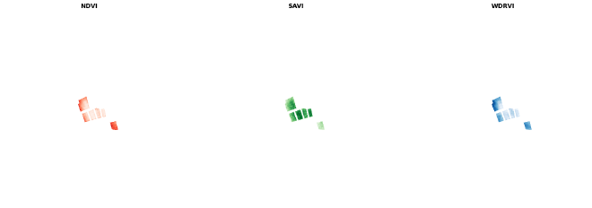
# 可视化
import matplotlib.pyplot as plt
from rasterio.plot import show 
fig, (ax1,ax2,ax3) = plt.subplots(figsize=[21,7], nrows=1,ncols=3)
show((datasets, Band_Names.index('NDVI')), ax=ax1,cmap='Reds',title='NDVI')
show((datasets, Band_Names.index('SAVI')), ax=ax2,cmap='Greens',title='SAVI')
show((datasets, Band_Names.index('WDRVI')), ax=ax3,cmap='Blues',title='WDRVI')
ax1.set_axis_off()
ax2.set_axis_off()
ax3.set_axis_off()
# fig.savefig("pred.png", bbox_inches='tight')
plt.show()

nir,red,green = rs.read(5),rs.read(3),rs.read(2)
def normalize(array):
    """Normalizes numpy arrays into scale 0.0 - 1.0"""
    array_min, array_max = array.min(), array.max()
    return ((array - array_min)/(array_max - array_min))
# 标准化
nirn,redn,greenn = normalize(nir),normalize(red),normalize(green)
# nirn,redn,greenn = nir,red,green

# 图像合成
nrg = np.dstack((nirn, redn, greenn))

# 设置背景
# Choose a threshold value
threshold = 0.1
# Create a mask for the background pixels
mask = (nirn < threshold) & (redn < threshold) & (greenn < threshold)
# Set the background pixels to white in the nrg array
nrg[mask] = (1,1,1)
# Display the image
plt.imshow(nrg)

# 导包
import rasterio as rio
from rasterio.plot import show
from sklearn import cluster
import matplotlib.pyplot as plt
import numpy as np
import matplotlib.colors as mc
# 读取数据
rs = rio.open('./data/planet_VIs.tif')  
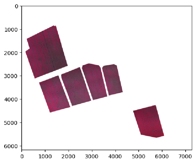
# 可视化
rs_data = rs.read() 
vmin, vmax = np.nanpercentile(rs_data, (2, 98))
plt.figure()
show(rs, vmin=vmin, vmax=vmax,cmap="gist_ncar")
plt.show()
# 数据预处理
rs_data_trans = rs_data.transpose(1,2,0)
rs_data.shape, rs_data_trans.shape
>> ((7, 694, 757), (694, 757, 7))
rs_data_1d = rs_data_trans.reshape(-1, rs_data_trans.shape[2])
rs_data_1d.shape
>> (525358, 7)
# 建模
cl = cluster.KMeans(n_clusters=4) # create an object of the classifier
param = cl.fit(rs_data_1d) # train it
# 输出
img_cl = cl.labels_ 
img_cl = img_cl.reshape(rs_data_trans[:,:,0].shape) 
# 保存结果
prof = rs.profile
prof.update(count=1)
with rio.open('result.tif','w',**prof) as dst:
    dst.write(img_cl, 1)
    
# 对比
fig, (ax1,ax2) = plt.subplots(figsize=[15,15], nrows=1,ncols=2)
show(rs, cmap='gray', vmin=vmin, vmax=vmax, ax=ax1)
show(img_cl, ax=ax2)
ax1.set_axis_off()
ax2.set_axis_off()
fig.savefig("pred.png", bbox_inches='tight')
plt.show()